Basic Ngspice Simulation with SkyWater PDK
I wanted to be able to use the simulation models from the SkyWater PDK to simulate my designs. This post details the process of getting a simple inverter simulation working as well as a surprise at the end.
SkyWater PDK
The SkyWater PDK can be found here. Unfortunately there is not much documentation at the moment so it can be hard to decipher where to start. The process of getting the PDK models is documented below
Installation
For the simulations you will need Ngspice installed. Go follow my tutorial for getting it installed here.
After Ngspice is installed, get the SkyWater PDK setup by running the following commands. These can be found on the main SkyWater PDK GitHub page here.
git clone https://github.com/google/skywater-pdk.git
cd skywater-pdk

# Expect a large download! ~7GB at time of writing.
SUBMODULE_VERSION=latest make submodules -j3 || make submodules -j1

# Regenerate liberty files
make timing
This will get all of the models and libraries included in the PDK. For just starting out you will probably only want the basic starting blocks.
In the libraries/ folder there are a bunch of folders that contain standard cells optimized for different use case. sky130_fd_sc_hd is for high density, sky130_fd_sc_hdll is for high density low leakage, sky130_fd_sc_hs is for high voltage, sky130_fd_sc_lp is for low power, you get the point.
We want the sky130_fd_pr folder which holds the primitives models and cells. In here there are capacitors, diodes, inductors, and more importantly for us, nfets and pfets.
I will be using the nfet_01v8 and pfet_01v8 cells which are just 1.8V optimized NMOS and PMOS transistors.
Ngspice Simulation
To get the simulation up and running, create new file named inv.cir and paste the following.
* SkyWater PDK
* simple inverter

.include "/home/philip/skywater-pdk/libraries/sky130_fd_pr/latest/models/corners/tt.spice"

* the voltage sources:
Vdd vdd gnd DC 1.8
V1 in gnd pulse(0 1.8 0p 200p 100p 1n 2n)

Xnot1 in vdd gnd out not1

.subckt not1 a vdd vss z
xm01   z a     vdd     vdd sky130_fd_pr__pfet_01v8_hvt  l=0.15  w=0.99  as=0.26235  ad=0.26235  ps=2.51   pd=2.51
xm02   z a     vss     vss sky130_fd_pr__nfet_01v8  l=0.15  w=0.495 as=0.131175 ad=0.131175 ps=1.52   pd=1.52
c3  a     vss   0.384f
c2  z     vss   0.576f
.ends

* simulation command:
.tran 1ps 10ns 0 10p

.control
run
plot in out
.endc
You will need to change the .include path to point to wherever you cloned the skywater-pdk folder.
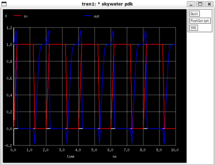
This circuit creates a simple CMOS inverter with a power supply voltage of 1V and a square wave input.
You might notice that the .include statement includes the tt.spice file. This file includes all of the Typical corner (tt) models for the cells in the sky130_fd_pr folder. There are other corner models like Slow-Fase (sf), Fast-Fast (ff), Slow-Slow (ss), Fast-Slow (fs), Low-Low (ll), High-High (hh), High-Low (hl), and Low-High (lh). You can include those models corresponding .spice file to run a simulation using that corner case.
To run the simulation, simply run Ngspice with the input file.
ngspice inv.cir
If everything is setup correctly you should see a plot like the one below showing the transient response of the inverter.

Congradulations! You have now simulated your first circuit using Ngspice and the SkyWater PDK. Now you can go and explore some of the other standard cells and corner models.
Suprise
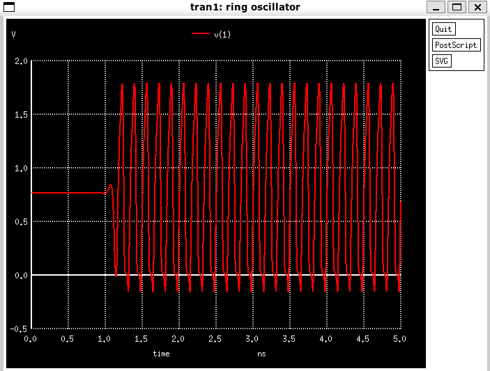
On this page, there is a simulation for a Ring Oscillator using inverters. I modified it slightly to get the simulation shown below.
Ring Oscillator
.include "/home/philip/skywater-pdk/libraries/sky130_fd_pr/latest/models/corners/tt.spice"

xinv1 1 2 vdd inv
xinv2 2 3 vdd inv
xinv3 3 1 vdd inv

vdd vdd 0 1.8

* Inverter block sub-circuit
.subckt inv vin vout vdd
	.param l = 0.15
	.param wp = 0.5
	.param wn = {wp * 1.5}

	xm1 vout vin 0 0 sky130_fd_pr__nfet_01v8 w=wn l=l
	xm2 vout vin vdd vdd sky130_fd_pr__pfet_01v8_hvt w=wp l=l
	*c1 vout 0 10f
.ends

.tran  1p 5n
.save v(1) v(2) v(3)

.control
run
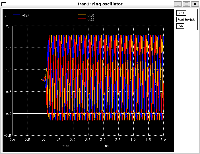
plot v(1) v(2) v(3)
.endc

.end
If you save this to a file and run (changing the .include path), you will see a simulation of a ring oscillator! The output plot is shown below.

