Simulating and2 Cells from SkyWater PDK
Here I wanted to try simulating some of the and2 cells that are provided by the SkyWater PDK. I also wanted to try out some of the Jupyter scripts that I wrote to read and plot the simulation data from Ngspice.
Simulating and2 Cells
I decided to simulate two of the and2 cells provided by the SkyWater PDK, specifically the sky130_fd_sc_hs__and2_1 and sky130_fd_sc_lp__and2_0 cells.
They are speed and power optimized versions of an AND gate.
These cells have a total of 7 connections. The regular A, B, and X logic inputs and outputs, Vgnd and Vpwr for power and ground, and Vnb and Vpb for the n-type and p-type body connections.
I chose to simulate the and2 cell with a 0.5fF load capacitor between the output and gnd. The logic inputs are connected to pulse sources and Vdd is set to 1V. Vnb is connected to gnd and Vpb is connected to Vdd.
I ran the simulation for 8ns to get 2 full cycles of all of the possible inputs to the and2 cell. The inputs are 00, 01, 10, and 11 so I only expect to get an output on the last one.
The spice file for the simulation is shown below. If you don’t already have Ngspice installed and the SkyWater PDK setup, read my post on Basic Ngspice Simulation with SkyWater PDK
and2 Transient Simulation
.include "/home/philip/skywater-pdk/libraries/sky130_fd_sc_hs/latest/cells/and2/sky130_fd_sc_hs__and2_1.spice"
.include "/home/philip/skywater-pdk/libraries/sky130_fd_sc_lp/latest/cells/and2/sky130_fd_sc_lp__and2_0.spice"
.include "/home/philip/skywater-pdk/libraries/sky130_fd_pr/latest/models/corners/tt.spice"


* High speed and2 cell
Vdd vdd gnd DC 1.0
V1 A gnd pulse(0 1.0 0p 100p 100p 1n 2n)
V2 B gnd pulse(0 1.0 1n 100p 100p 2n 4n)

X1 A B gnd gnd Vdd Vdd out sky130_fd_sc_hs__and2_1
c1 out gnd 0.5f


* Low power and2 cell
Vdd2 vdd2 gnd DC 1.0
V12 A2 gnd pulse(0 1.0 0p 100p 100p 1n 2n)
V22 B2 gnd pulse(0 1.0 1n 100p 100p 2n 4n)

X2 A2 B2 gnd gnd Vdd2 Vdd2 out2 sky130_fd_sc_lp__and2_0
c2 out2 gnd 0.5f


* simulation command:
.tran 1ps 8ns 0 10p

.save A B out
.save A2 B2 out2
.save i(Vdd)
.save i(Vdd2)

.control
run

plot A B out
plot A2 B2 out2

plot i(Vdd)
plot i(Vdd2)
.endc

.end
I used Ngspice to simulate and output the raw data to a file using the following command
ngspice -b -r and2.raw and2.cir
To view the graphs using the built-in waveform viewer use the command below.
ngspice and2.cir
Plotting Data
Now that I have the raw simulation data, I used a Jupyter notebook and Matplotlib to graph the data.
To read from the simulation output file I used the LTspice pytool library which reads in the binary .raw files that Ngspice outputs into python.
Originally this library was written for LTspice (hence the name), but with a slight modification it can also read Ngspice .raw files.
The Jupyter notebook code I used to create the graphs is shown at the end. All it does is read in the data and plot it on a nicely formatted plot.
Show below is a plot of the input voltages as well as the resulting output voltage vs time.
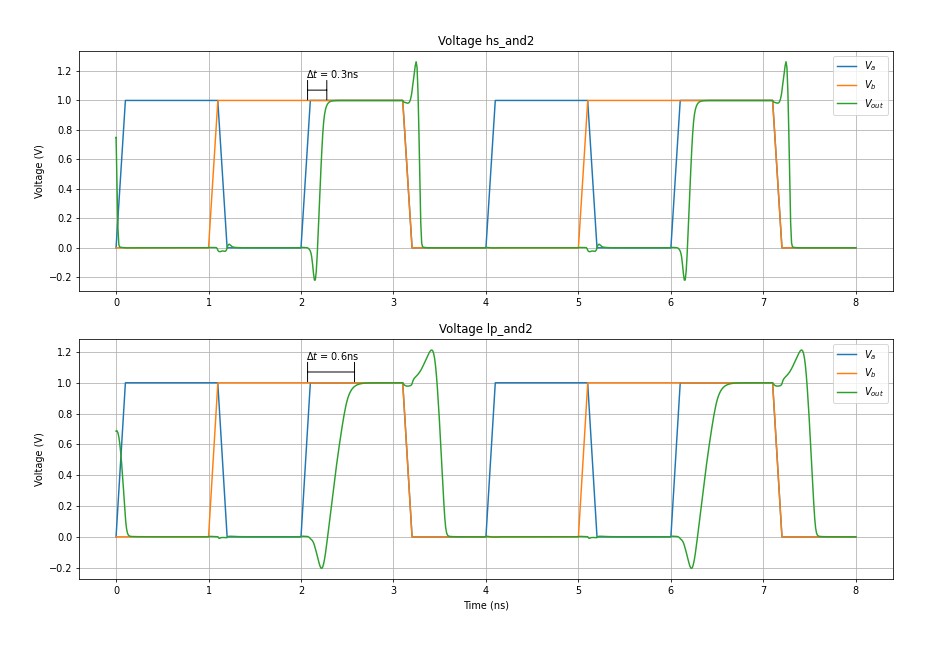
Now I can directly compare the differences in propagation delay between the speed optimized gate and the power optimized gate.
I can also plot the current supplied by Vdd vs time.
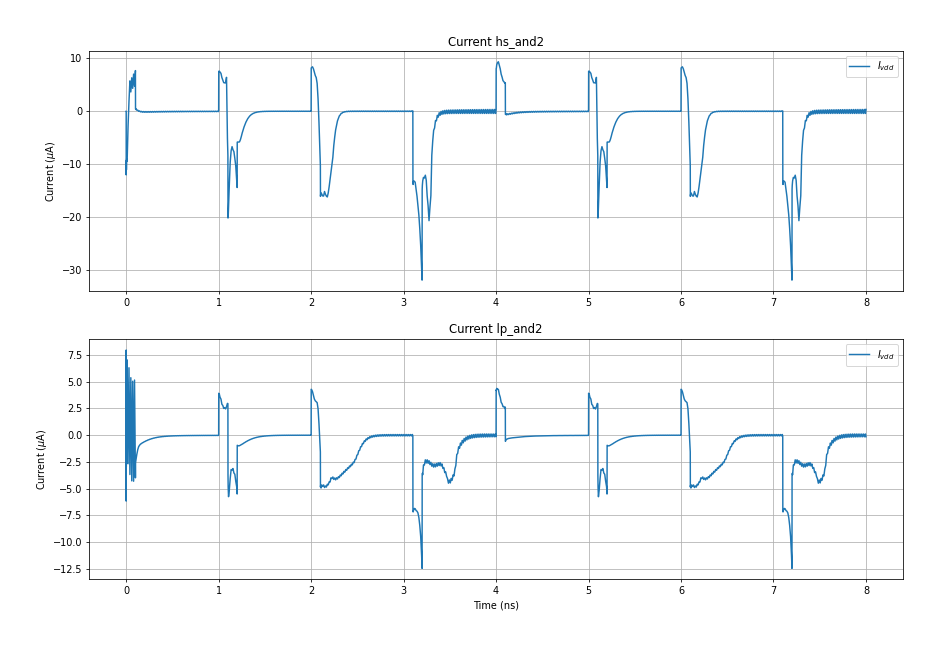
A thing to notice is the difference in the heights of the current spikes between the two designs.
Since I have the data loaded in the Jupyter notebook, I can do any other calculations that I might want to do. This makes it rather easy to do analysis on any sorts of simulations that you might do in Ngspice.
Jupyter Code
import ltspice
from matplotlib import pyplot as plt
import numpy as np
import os

%matplotlib inline

# -------------------------------
# Reading in data from simulation
# -------------------------------

l = ltspice.Ltspice(os.path.abspath('') + '/and2.raw').set_variable_dtype(float)
# Make sure that the .raw file is located in the correct path
l.parse()

time = l.get_time() * 1E9 # Convert time to nanoseconds
V_a = l.get_data('V(A)')
V_b = l.get_data('V(B)')
V_out = l.get_data('V(out)')

V_a2 = l.get_data('V(A2)')
V_b2 = l.get_data('V(B2)')
V_out2 = l.get_data('V(out2)')

I_vdd = l.get_data('i(Vdd)') * 1E6 # Convert time to microseconds
I_vdd2= l.get_data('i(Vdd2)') * 1E6

I_vdd[:4] = 0 # Weird artifact at beginning of simulation
I_vdd2[:4] = 0

plt.rcParams['figure.figsize'] = [15, 10]

# ----------------------
# Plotting voltage graph
# ----------------------

fig, axs = plt.subplots(2, 1, gridspec_kw = {'hspace':0.2})

axs[0].plot(time, V_a, label='$V_{a}$')
axs[0].plot(time, V_b, label='$V_{b}$')
axs[0].plot(time, V_out, label='$V_{out}$')
axs[0].set_title('Voltage hs_and2')
axs[0].set(ylabel='Voltage (V)')
axs[0].annotate('$\Delta t$ = 0.3ns', xy=(2.05, 1.15))
axs[0].annotate("",
            xy=(2.05, 1.07), xycoords='data',
            xytext=(2.3, 1.07), textcoords='data',
            arrowprops=dict(arrowstyle="|-|",
                            connectionstyle="arc3,rad=0"),
            )

axs[1].plot(time, V_a2, label='$V_{a}$')
axs[1].plot(time, V_b2, label='$V_{b}$')
axs[1].plot(time, V_out2, label='$V_{out}$')
axs[1].set_title('Voltage lp_and2')
axs[1].set(xlabel='Time (ns)', ylabel='Voltage (V)')
axs[1].annotate('$\Delta t$ = 0.6ns', xy=(2.05, 1.15))
axs[1].annotate("",
            xy=(2.05, 1.07), xycoords='data',
            xytext=(2.6, 1.07), textcoords='data',
            arrowprops=dict(arrowstyle="|-|",
                            connectionstyle="arc3,rad=0"),
            )

for ax in axs.flat:
    ax.grid()
    ax.legend()

fig.savefig('and2-voltage.png', facecolor="w", dpi=70, bbox_inches='tight', pad_inches=0.5)

# ----------------------
# Plotting current graph
# ----------------------

fig, axs = plt.subplots(2, 1, gridspec_kw = {'hspace':0.2})

axs[0].plot(time, I_vdd, label='$I_{vdd}$')
axs[0].set_title('Current hs_and2')
axs[0].set(ylabel='Current ($\mu$A)')

axs[1].plot(time, I_vdd2, label='$I_{vdd}$')
axs[1].set_title('Current lp_and2')
axs[1].set(xlabel='Time (ns)', ylabel='Current ($\mu$A)')

for ax in axs.flat:
    ax.grid()
    ax.legend()

fig.savefig('and2-current.png', facecolor="w", dpi=70, bbox_inches='tight', pad_inches=0.5)