DC Transfer Function of an Inverter using SkyWater PDK
I wanted to be able to plot the DC transfer function of a inverter and vary the width of the mosfet gate to see the effect that it has on the threshold voltage. Hopefully the results from the simulation models should match the theory.
Simulating an inverter
To simulate an inverter, I started with a nfet and a pfet.
I used the sky130_fd_pr__nfet_01v8 and sky130_fd_pr__pfet_01v8 cells that are provided as part of the SkyWater PDK in the sky130_fd_pr library.
These were connected to form an inverter in a subcircuit. The subcircuit just allows for easier use of the inverter when it is used in larger designs and isn’t strictly necessary here.
I also connected one voltage source, vs, to the input of the inverter and a second voltage source, vdd, to power the inverter.
I set the length of both inverters to \(0.2 \mu \text{m}\). I set the length of the nfet to \(1 \mu \text{m}\) since that is where I am going to start the sweep of the length of the pfet.
I am sweeping the width of the pfet from \(1 \mu \text{m}\) to \(10 \mu \text{m}\). This will produce a nice range of widths to see the variation of the DC transfer function.
The spice file describing the simulation is shown below. You will need to change the path of the .include to point to wherever you have installed the SkyWater PDK.
If you don’t already have Ngspice installed and the SkyWater PDK setup, read my post on Basic Ngspice Simulation with SkyWater PDK.
Inverter DC Transfer

.include "/home/philip/skywater-pdk/libraries/sky130_fd_pr/latest/models/corners/tt.spice"

* the voltage sources:
vs  in  0 dc 1.8
vdd vdd 0 dc 1.8

Xnot1 in vdd 0 out not1

.subckt not1 a vdd vss z
    .param width = 0.5
    xm01 z a vdd vdd sky130_fd_pr__pfet_01v8  l=0.2  w=width
    xm02 z a vss vss sky130_fd_pr__nfet_01v8  l=0.2  w=1
.ends

.control

    let nmoswidth = 1
    alterparam not1 width=$&nmoswidth
    reset
    let cnt = 0
    dowhile cnt < 10
        dc vs 0 1.8 0.001
        write data/inverter-{$&nmoswidth}.raw
        let nmoswidth = nmoswidth + 1
        alterparam not1 width=$&nmoswidth
        reset
        let cnt = cnt + 1
    end

    plot dc1.out dc2.out dc3.out dc4.out dc5.out dc6.out xlabel "input voltage (V)" ylabel "output voltage (V)"  title "DC Transfer of Inverter as function of pfet width"

.endc
This simulation writes the raw data to a .raw file for each variation of the width of the pfet. For this to work, a folder named data has to exist in the same folder where the simulation is run.
If you run Ngspice in interactive mode, you should see a plot something like the one below.
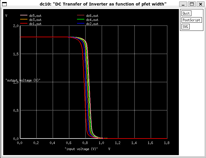
It can be quite hard to actually analyze the data using the built in waveform viewer but do not worry, Python is here to the rescue!
Making Better Plots
I am using a Jupyter notebook and the raw files output by the simulation to create nicer looking plots. It will also be easier to analyze the data and extract the circuit performance parameters from the data in python.
I am using the library ltspice to read in the raw binary data from Ngspice. I can then plot the data on a plot using Matplotlib and format it nicely so that it is easier to see.
The output plot can be seen below.
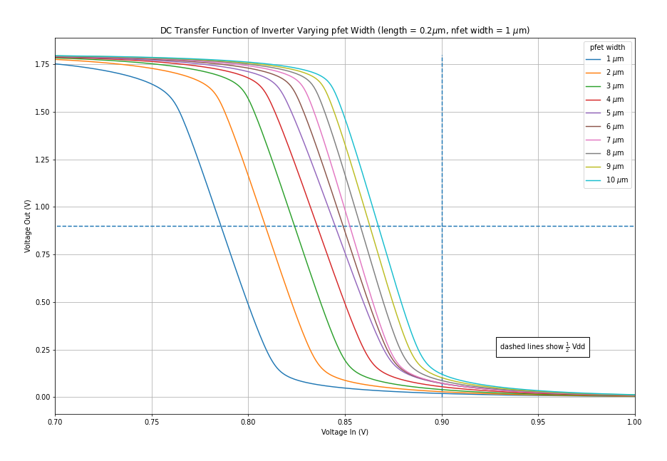
Now it is easier to see how the inverter threshold voltage changes as the pfet width changes.
Jupyter Notebook Code
The code will read in any .raw files that are in the data/ folder and try to parse and read v(in) and v(out).
This makes it rather easy to add more or less variations of the width.
The notebook should be run from the same folder that the Ngspice simulation is run in so that it can find the data/ folder containing the raw output from the simulations.
import ltspice
from matplotlib import pyplot as plt
import numpy as np
import os
from os import walk
import re

%matplotlib inline

dir_name = os.path.abspath('') + '/data'
filenames = next(walk(dir_name), (None, None, []))[2]  # [] if no file
filenames.sort(key=lambda f: int(re.sub('\D', '', f)))

labels = []
voltage_in = []
voltage_out = []

for filename in filenames:
    label = (filename.split('inverter-'))[1].split('.raw')[0]
    labels.append(label + " $$0.2 \mu \text{m}$$")

    l = ltspice.Ltspice(os.path.abspath('') + '/data/' + filename).set_variable_dtype(float)
    l.parse()

    voltage_in.append(l.get_data('v(in)'))
    voltage_out.append(l.get_data('v(out)'))

plt.rcParams['figure.figsize'] = [15, 10]

for voltage, label in zip(voltage_out, labels):
    plt.plot(voltage_in[0], voltage, label=label)

plt.title('DC Transfer Function of Inverter Varying pfet Width (length = 0.2$$0.2 \mu \text{m}$$, nfet width = 1 $$0.2 \mu \text{m}$$)')
plt.xlabel('Voltage In (V)')
plt.ylabel('Voltage Out (V)')
plt.legend(title='pfet width')
plt.xlim([0.7, 1])

plt.vlines(0.9, 0, 1.8, linestyles='dashed')
plt.hlines(0.9, 0, 1.8, linestyles='dashed')

plt.text(0.93, 0.25, 'dashed lines show $\\frac{1}{2}$ Vdd',
        bbox={'facecolor': 'white','edgecolor' : 'black', 'pad': 5})

plt.grid()

plt.savefig('python-dc-transfer.png', facecolor="w", dpi=70, bbox_inches='tight', pad_inches=0.5)